Incorporating a broad line fit
Contributor: Julia Falcone
Targets such as Seyfert 1 galaxies possess both broad and narrow lines. However, whereas narrow line components are relatively free to scale in various ways depending on the data and the number of narrow line components may change from one position to the next, the number of broad line components and the fluxes of the broad line components relative to each other are fixed. Thus, you only have to solve for the broad component once, and then it can be reapplied to the rest of the data in your data set.
There are two ways we can go about solving for the broad components. You are free to follow along in the example Jupyer notebook:
Method 1: Fit Everything at Once
The most straightforward method would be to fit broad and narrow lines simultaneously, and then extract the broad line components from the results. The parameters are shown in the example Jupyter notebook under the same heading as this subsection. Note that the mindiwth and maxwidth are 1 Å and 50 Å, respectively, and that maxcomp is 5. See [other page] to read more about how to determine these values for your own data. Note that this method can become computationally expensive, as each additional fitted component requires an exponential increase in resources.
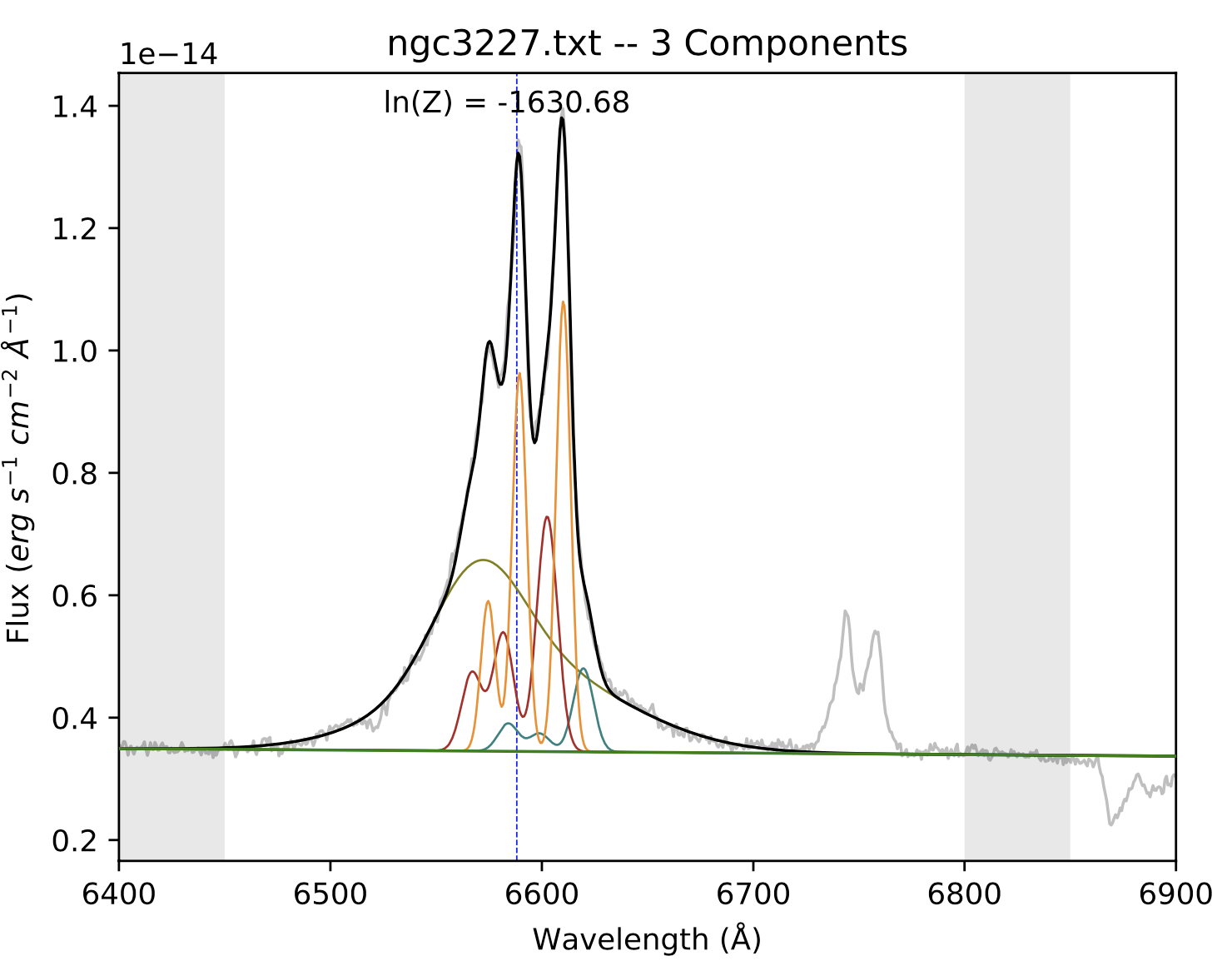
The resulting best fit is shown below, along with the output parameters.
Line color |
Wavelength centroid |
Width |
Flux |
|---|---|---|---|
Blue/teal |
6587 |
6.1 |
4.14E-14 |
Pink |
6589 |
2.1 |
1.89E-14 |
Orange (tall) |
6579 |
25.8 |
1.83E-13 |
Orange (short) |
6585 |
50 |
3.75E-14 |
The two orange curves are the broad components, and so those parameters form the basis of the prefit_instructions for all the other fits of these lines in this data set.
Method 2: Use an Iterative Prodecure
Step 1: Fitting only the broad lines
In our first example fit which had only narrow lines in its spectrum, we allowed BEAT to fit lines of any width up to a maxwidth of 5 Å (corresponding to ~230 km/s). Because the narrow lines are fairly well constrained in their widths, as long as the maxwidth is above the values of the widths, the fit will also be well constrined.
However, the maxwidth value has more significance when we introduce a spectrum with broad and narrow lines. The first part of this process will involve only fitting the broad line(s). It will be done once to a single spectrum in your data set, and then those resulting Gaussians will be applied to the rest of the spectra when fitting the narrow lines.
The first step is to run BEAT on your spectrum, where the minwidth is now 15 Å and the maxwidth can be a significantly value like 50 Å. It will likely produce a three-component fit with similar parameters as shown below. It might be puzzling that we allow the maxwidth of narrow lines to only go up to 5 Å, whereas the broad lines have a minwidth of 15 Å. What about the lines in the middle, with a width of 5 - 15 Å? Such lines belong to the intermediate line region (IRL), whose emission lines are semi-blended. Kinematic studies can reveal whether your target has a prevalent ILR, and in the case of this specific example (NGC 3227), it does not. Please note that these values for the widths are rough estimates, and may not apply in exactly the same way to your target(s).
Line color |
Wavelength centroid [Å] |
Width [Å] |
Flux [erg s-1 cm-2 Å-1] |
|---|---|---|---|
Blue/teal |
6629 |
50 |
2.42E-14 |
Pink |
6570 |
34.1 |
9.80E-14 |
Orange |
6582 |
15 |
8.92E-14 |
In the above image, the blue curve is clearly trying to fit the narrow components. Therefore, we determine that our first estimate of the broad components are the orange and pink fits, whose parameters are shown in the table above. To understand how we extracted the parameters for the table, please look at the Interpreting the output page.
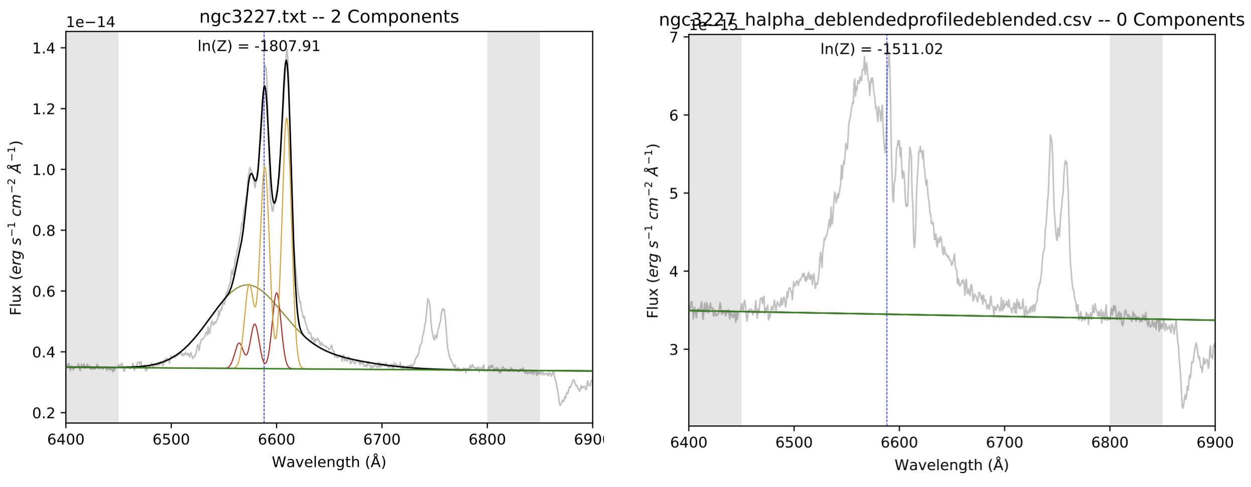
Step 2: Fitting the spectrum with new broad parameters
In this step, will be fitting narrow lines to our spectrum using the broad components that we just found in Step 1. We copy the parameters from the pink and orange curves into prefit_instructions, calculating the flux ratio from the fluxes, and reset the minwidth and maxwidth parameters back to 1.5 Å and 5 Å, respectively.
Notice how, in the fit = beat.Fit section of the code, there is a new parameter that reads save_NLR_removed = True. This is because once BEAT fits the narrow components to the spectrum, it will then subtract those components from the data, thereby isolating the broad region. The left image below is the final fit from this BEAT run. It’s evident that this broad region still needs some improvement, as it looks unusually shifted to the left, but this isn’t concerning because the fit will improve with each iteration. On the right is the spectrum in the NLR_removed directory that is created in the output, which has subtracted the two narrow line components in the left image from the data. The spectrum is pretty jagged, but this can also improve with future iterations.
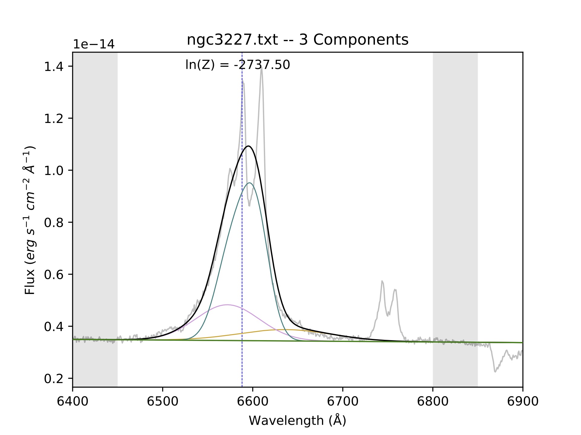
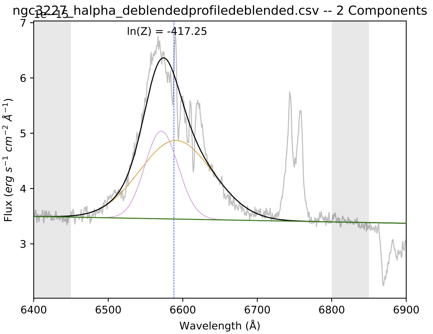
Step 3: Fitting the NLR-subtracted spectrum
In this round of fitting, we are going to use the same maxwidth and minwidth that we used for Step 1. This is because we’re fitting the NLR-subtracted spectrum seen in the right-hand image of the last step. If we assume the broad region is isolated with this spectrum, we can limit ourselves to only fiting broad lines. Note that spec_dir should now point to the NLR_removed directory that was produced in the previous step. The image below shows the resulting fit to this spectrum.
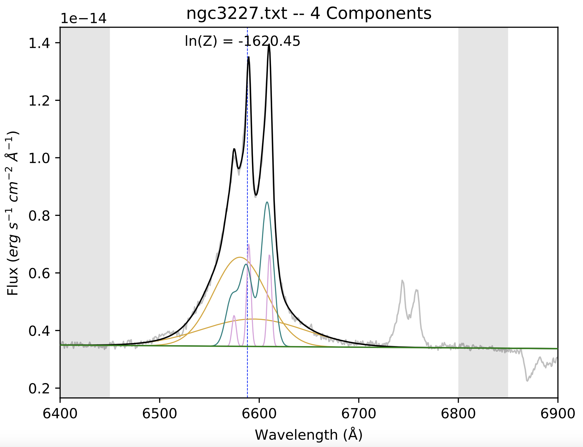
Step 4: Fitting the spectrum with newer broad parameters
Now that I have an improved set of broad parameters, we can put them back into the prefit_instructions and once again reset our minwidth and maxwidth to identify narrow lines (i.e., set them to 1.5 Å and 5 Å, respectively).
The figure above shows our resulting 3-component fit that accurately models both the broad- and narrow-line region. Steps 3 and 4 could be repeated again, but more iterations does not necessarily result in a better fit. To know whether successive iterations are better fits than previous ones, you should compare the fits’ ln(Z) values. For more information about the ln(Z) parameter, see Feroz et al. 2011 and Section 3.1 of Falcone et al. 2024
Once you are satisfied with the quality of this fit, the broad region parameters– which are to say, the output parameters that you get from Step 3– can then be implemented into the prefit_instructions for all fits of this dataset going forward. Note that the ln(z) values for the final step of this method and that of Method 1 are very close, indicating a similar quality of the fits. In other words, either method is equally adequate to reach a proper broad line fit.